CHAPTER 9 PYTHON LIBRARY SERIES-PANDAS

 A well-liked open-source Python data manipulation and analysis library is called pandas. It offers the user-friendly functionalities and data structures required to work with structured data with ease. The following are some essential features of the pandas library and their importance:

Data Frame and Data Series:

Data Frame: The Data Frame, a two-dimensional table with rows and columns, is the main data structure in pandas. It makes it possible for you to effectively store and handle labeled, structured data.

Series: Any kind of data can be stored in this one-dimensional labelled array. The fundamental units of Data Frames are series.

Cleaning and Data Preparation:

Pandas offers strong data preparation and cleaning tools. It has tools for dealing with missing data, rearranging data, and changing the sorts of data.

To handle missing or inaccurate data, methods like dropna(), fillna(), and replace() are frequently utilized.

Data Analysis and Exploration: With the use of summary functions and descriptive statistics, Pandas makes it simple to explore data. For numerical columns, the describe() technique yields statistical summaries; for categorical data, value_counts() is helpful.

Pandas makes it simple to group, aggregate, and filter data, facilitating effective data analysis.

Time Series Analysis: Time series data is well supported by Pandas. It is ideal for studying time-dependent data since it offers capabilities for resampling, time-based indexing, and moving window statistics.

Data joining and merging: In data analysis, combining data from many sources is a frequent operation. Pandas has a number of join and merge functions, including concat() and merge().

Data Input/Output: Pandas can read and write data in a number of different forms, such as Excel, CSV, SQL databases, JSON, and more. Data import and export between sources is now simple as a result.

Flexibility and Performance:

Pandas is made to be user-friendly and flexible. It offers complex functions for more experienced users, but also makes data manipulation accessible to newcomers with its high-level interface.

Python is based on NumPy, a high-performance numerical computing toolkit, internally. This guarantees effective data processing, particularly with regard to big datasets.

Combining with Different Libraries:

NumPy, Matplotlib, Seaborn, scikit-learn, and other data science and machine learning libraries in the Python environment are among the libraries with which Pandas interacts well. A thorough and effective data analysis procedure is made possible by this flawless connection.

Acquiring knowledge of the Pandas library in Python can be beneficial for manipulating data, particularly in data science and analysis activities. Pandas offers a range of methods for data manipulation, cleaning, and analysis in addition to data structures like Data Frames and Series. Here's a step-by-step tutorial to get you started learning about pandas:

To get data file, kindly click here: 

https://drive.google.com/drive/folders/1O6OFRmHvCEP6KmFDUlEOTuKBAth0K4ao?usp=sharing

. Install Pandas:

Make sure you have Python installed on your system. You can install Pandas using pip:

pip install pandas

2. Import Pandas:

In your Python script or Jupyter notebook, import the Pandas library:

import pandas as pd

3. Data Structures:

a. Series:

A one-dimensional array-like object. You can create a Series from a list, array, or dictionary.

student_marks = [67, 28, 83, 64]

s = pd.Series(student_marks)

print(s)

Output:

0    67

1    28

2    83

3    64

dtype: int64

 

b. DataFrame:

A two-dimensional table of data with rows and columns. 

You can create a DataFrame from a dictionary, NumPy array, or 

other data structures.

weather_data = {'Month': ['Jan', 'Feb', ‘Mar’],

        'Temp': [25, 30, 35],

        'Town': ['San Francisco', 'New York', 'Los Angeles']}

df_new= pd.DataFrame(weather_data)

print(df_new)

Output:

   Month  Temp           Town

0    Jan    25  San Francisco

1    Feb    30       New York

2  March    35    Los Angeles

 

4. Reading Data:

Read data from various sources like CSV, Excel, SQL databases, etc.

# CSV

df = pd.read_csv('your_data.csv')

# Excel

df = pd.read_excel('your_data.xlsx')

5. Exploring Data:

Useful functions to explore your data:

# Display basic information about the DataFrame

df.info()

# Summary statistics

df.describe()

# Display the first few rows

df.head()

# Display the last few rows

df.tail()

Practice:

import pandas as pd

# To read the CSV file as a dataframe

file_path=('Lucknow_1990_2022.csv')

df = pd.read_csv('D:\Education Content-2\Apple\Books\pyhthon folder\Lucknow_1990_2022.csv')

# To get few rows of the DataFrame

print(df.head())

# To get basic information of the dataframe.

print(df.info())

# To display the summary statistics of all numerical columns

print(df.describe())

Output:

time  tavg  tmin  tmax  prcp

0  01-01-1990   7.2   NaN  18.1   0.0

1  02-01-1990  10.5   NaN  17.2   0.0

2  03-01-1990  10.2   1.8  18.6   NaN

3  04-01-1990   9.1   NaN  19.3   0.0

4  05-01-1990  13.5   NaN  23.8   0.0

<class 'pandas.core.frame.DataFrame'>

RangeIndex: 11894 entries, 0 to 11893

Data columns (total 5 columns):

 #   Column  Non-Null Count  Dtype  

---  ------  --------------  -----  

 0   time    11894 non-null  object 

 1   tavg    11756 non-null  float64

 2   tmin    8379 non-null   float64

 3   tmax    10341 non-null  float64

 4   prcp    5742 non-null   float64

dtypes: float64(4), object(1)

memory usage: 464.7+ KB

None

               tavg         tmin          tmax         prcp

count  11756.000000  8379.000000  10341.000000  5742.000000

mean      25.221240    18.795859     32.493405     4.535650

std        6.717716     7.197118      6.214145    17.079051

min        5.700000    -0.600000     11.100000     0.000000

25%       19.500000    12.500000     28.100000     0.000000

50%       27.200000    20.500000     33.400000     0.000000

75%       30.400000    25.100000     36.500000     1.000000

max       39.700000    32.700000     47.300000   470.900000

 

To get the CSV file used here, click the link: 

import pandas as pd

# To read the CSV file as a dataframe

file_path=('Lucknow_1990_2022.csv')

df = pd.read_csv('D:\Education Content-2\Apple\Books\pyhthon folder\Lucknow_1990_2022.csv')

# To get few rows of the DataFrame

print(df.head())

# To get basic information of the dataframe.

print(df.info())

# To display the summary statistics of all numerical columns

print(df.describe())

 

Output:

  time  tavg  tmin  tmax  prcp

0  01-01-1990   7.2   NaN  18.1   0.0

1  02-01-1990  10.5   NaN  17.2   0.0

2  03-01-1990  10.2   1.8  18.6   NaN

3  04-01-1990   9.1   NaN  19.3   0.0

4  05-01-1990  13.5   NaN  23.8   0.0

<class 'pandas.core.frame.DataFrame'>

RangeIndex: 11894 entries, 0 to 11893

Data columns (total 5 columns):

 #   Column  Non-Null Count  Dtype 

---  ------  --------------  ----- 

 0   time    11894 non-null  object

 1   tavg    11756 non-null  float64

 2   tmin    8379 non-null   float64

 3   tmax    10341 non-null  float64

 4   prcp    5742 non-null   float64

dtypes: float64(4), object(1)

memory usage: 464.7+ KB

None

               tavg         tmin          tmax         prcp

count  11756.000000  8379.000000  10341.000000  5742.000000

mean      25.221240    18.795859     32.493405     4.535650

std        6.717716     7.197118      6.214145    17.079051

min        5.700000    -0.600000     11.100000     0.000000

25%       19.500000    12.500000     28.100000     0.000000

50%       27.200000    20.500000     33.400000     0.000000

75%       30.400000    25.100000     36.500000     1.000000

max       39.700000    32.700000     47.300000   470.900000

 

6. Data Manipulation:

a. Selection and Filtering:

# Selecting a column

df['Name']

column_read=df['tavg']

print(column_read)

Output:

0         7.2

1        10.5

2        10.2

3         9.1

4        13.5

         ...

11889    27.4

11890    28.1

11891    30.3

11892    30.0

11893    27.1

Name: tavg, Length: 11894, dtype: float64

Output:

# Selecting multiple columns

df[['Name', 'Age']] #sample code, it is not executed.

column_read=df[['tavg','tmin']]

print(column_read)

Output:

        tavg  tmin

0       7.2   NaN

1      10.5   NaN

2      10.2   1.8

3       9.1   NaN

4      13.5   NaN

...     ...   ...

11889  27.4  25.1

11890  28.1  26.1

11891  30.3  26.2

11892  30.0  28.1

11893  27.1  24.1

[11894 rows x 2 columns]

# Filtering rows

df[df['Age'] > 30] #sample code, it is not executed.

filtered_df = df[df['tavg'] > 20]

print(filtered_df)

Output:

 

             time  tavg  tmin  tmax  prcp

18     19-01-1990  20.5  13.0  29.5   NaN

27     28-01-1990  20.7   NaN  28.8   0.0

28     29-01-1990  21.4   NaN  28.8   0.0

37     07-02-1990  20.7  10.1  25.9   0.0

38     08-02-1990  20.7  12.9  26.1   NaN

...           ...   ...   ...   ...   ...

11889  21-07-2022  27.4  25.1  33.1  27.3

11890  22-07-2022  28.1  26.1  31.1  16.0

11891  23-07-2022  30.3  26.2  34.7  11.9

11892  24-07-2022  30.0  28.1  34.7   2.0

11893  25-07-2022  27.1  24.1  34.3   0.5

 

[8577 rows x 5 columns]

b. Adding and Removing Columns:

# Adding a new column

df['NewColumn'] = df['Age'] * 2

#sample code, it is not executed.

# Removing a column

df.drop('NewColumn', axis=1, inplace=True)

c. Handling Missing Data:

# Check for missing values

df.isnull().sum()

 

# Drop rows with missing values

df.dropna()

 

# Fill missing values

df.fillna(value)

7. Grouping and Aggregation:

 

# Group by a column and calculate mean

df.groupby('City')['Age'].mean()

 

import pandas as pd

# To read the CSV file as a dataframe

file_path=('Lucknow_1990_2022.csv')

df = pd.read_csv('D:\Education Content-2\Apple\Books\pyhthon folder\Lucknow_1990_2022.csv')

# To get few rows of the DataFrame

print(df.head())

# To get basic information of the dataframe.

print(df.info())

# To display the summary statistics of all numerical columns

print(df.describe())

df_filled = df.fillna(value=0)

OUTPUT:

         time  tavg  tmin  tmax  prcp

0  01-01-1990   7.2   NaN  18.1   0.0

1  02-01-1990  10.5   NaN  17.2   0.0

2  03-01-1990  10.2   1.8  18.6   NaN

3  04-01-1990   9.1   NaN  19.3   0.0

4  05-01-1990  13.5   NaN  23.8   0.0

<class 'pandas.core.frame.DataFrame'>

RangeIndex: 11894 entries, 0 to 11893

Data columns (total 5 columns):

 #   Column  Non-Null Count  Dtype  

---  ------  --------------  -----  

 0   time    11894 non-null  object 

 1   tavg    11756 non-null  float64

 2   tmin    8379 non-null   float64

 3   tmax    10341 non-null  float64

 4   prcp    5742 non-null   float64

dtypes: float64(4), object(1)

memory usage: 464.7+ KB

None

               tavg         tmin          tmax         prcp

count  11756.000000  8379.000000  10341.000000  5742.000000

mean      25.221240    18.795859     32.493405     4.535650

std        6.717716     7.197118      6.214145    17.079051

min        5.700000    -0.600000     11.100000     0.000000

25%       19.500000    12.500000     28.100000     0.000000

50%       27.200000    20.500000     33.400000     0.000000

75%       30.400000    25.100000     36.500000     1.000000

max       39.700000    32.700000     47.300000   470.900000

 

# Grouping data by a column and calculating mean

grouped_df = df.groupby('time')['tavg'].mean()

grouped_df

OUTPUT:

time

01-01-1990     7.2

01-01-1991    11.5

01-01-1992     9.9

01-01-1993    14.4

01-01-1994    14.0

              ...

31-12-2017    12.4

31-12-2018    13.3

31-12-2019     8.4

31-12-2020     9.9

31-12-2021    13.9

Name: tavg, Length: 11894, dtype: float64

 

# Aggregating data with multiple functions

agg_df = df.groupby('time').agg({'tavg': ['mean', 'sum']})

agg_df

grouped_df.size

OUTPUT:

tavg
	mean	sum
time
01-01-1990	7.2	7.2
01-01-1991	11.5	11.5
01-01-1992	9.9	9.9
01-01-1993	14.4	14.4
01-01-1994	14.0	14.0
...	...	...
31-12-2017	12.4	12.4
31-12-2018	13.3	13.3
31-12-2019	8.4	8.4
31-12-2020	9.9	9.9
31-12-2021	13.9	13.9

11894 rows × 2 columns

 

grouped_df.size

OUTPUT:

11894

grouped_df.index

OUTPUT:

Index(['01-01-1990', '01-01-1991', '01-01-1992', '01-01-1993', '01-01-1994',

       '01-01-1995', '01-01-1996', '01-01-1997', '01-01-1998', '01-01-1999',

       ...

       '31-12-2012', '31-12-2013', '31-12-2014', '31-12-2015', '31-12-2016',

       '31-12-2017', '31-12-2018', '31-12-2019', '31-12-2020', '31-12-2021'],

      dtype='object', name='time', length=11894)

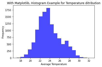
8. Data Visualization:

Pandas integrates well with Matplotlib and Seaborn for data visualization:

import matplotlib.pyplot as plt

import seaborn as sns

# Histogram

import matplotlib.pyplot as plt

df['tavg'].hist()

plt.show()

OUTPUT:

# Scatter plot

import seaborn as sns

sns.scatterplot(x='tmin', y='tmax', data=df)

plt.show()

OUTPUT:

9. Practice:

#The manager calls the Analytical Engineer to go through the following data thoroughly and then answer the questions asked.

a)Which day has the highest average temperature? 10-06-2014 

b)Which day has the lowest average temperature? 07-02-2008 

import pandas as pd

# To read the CSV file as a dataframe

file_path=('Mumbai_1990_2022_Santacruz.csv')

df = pd.read_csv('D:\Education Content-2\Apple\Books\pyhthon folder\Mumbai_1990_2022_Santacruz.csv')

#To find the maximum average value

tmax1='tavg'

max_value=df[tmax1].max()

print(max_value)

maxvalue_row=df.loc[df[tmax1] ==max_value]

print(maxvalue_row)

#To find the minimum average value

tmin1='tavg' # repeat the same step as done for ‘max_value’

min_value=df[tmin1].min()

print(min_value)

minvalue_row=df.loc[df[tmin1]==min_value]

print(minvalue_row)

 

OUTPUT:

33.7

            time  tavg  tmin  tmax  prcp

8926  10-06-2014  33.7   NaN   NaN   NaN

 

17.7

            time  tavg  tmin  tmax  prcp

6611  07-02-2008  17.7   NaN  23.2   NaN

 

How much data is there in this data base, before and after cleaning the data?

nan_value=df.isna()

print(nan_value)

#drop row which hold nan value

df_filled=df.dropna()

print(df_filled)

 

OUTPUT:

       time   tavg   tmin   tmax   prcp

0      False  False  False   True  False

1      False  False  False  False  False

2      False  False  False  False  False

3      False  False  False  False  False

4      False  False  False  False  False

...      ...    ...    ...    ...    ...

11889  False  False  False  False  False

11890  False  False  False  False  False

11891  False  False  False  False  False

11892  False  False  False  False  False

11893  False  False  False  False  False

 

[11894 rows x 5 columns]

 

            time  tavg  tmin  tmax  prcp

1      02-01-1990  22.2  16.5  29.9   0.0

2      03-01-1990  21.8  16.3  30.7   0.0

3      04-01-1990  25.4  17.9  31.8   0.0

4      05-01-1990  26.5  19.3  33.7   0.0

5      06-01-1990  25.1  19.8  33.5   0.0

...           ...   ...   ...   ...   ...

11889  21-07-2022  27.6  25.6  30.5  10.9

11890  22-07-2022  28.3  26.0  30.5   3.0

11891  23-07-2022  28.2  25.8  31.3   5.1

11892  24-07-2022  28.1  25.6  30.4   7.1

11893  25-07-2022  28.3  25.1  30.2   7.1

 

[4623 rows x 5 columns]

 

 

 

Which day recorded the lowest temperature? 08-02-2008 

#To find the minimum average value

tmin1='tmin' # repeat the same step as done for ‘tmax’ column

min_value=df[tmin1].min()

print(min_value)

minvalue_row=df.loc[df[tmin1]==min_value]

print(minvalue_row)

 

OUTPUT:

8.5

            time  tavg  tmin  tmax  prcp

6612  08-02-2008  17.9   8.5  22.3   NaN

 

Which day recorded the highest temperature? 16-03-2011 

tmax_value='tmax'

tmax_value1=df[tmax_value].max()

print(tmax_value1)

OUTPUT:

41.3

tmax_row=df.loc[df[tmax_value]==tmax_value1]

print(tmax_row)

            time           tavg  tmin  tmax  prcp

7744  16-03-2011  32.8  19.2  41.3   NaN

 

CHAPTER 8 PYTHON LIBRARY SERIES- MATPLOTLIB

A well-known Python library for producing interactive, animated, and static visualizations in a range of formats is called Matplotlib. It is appropriate for a variety of data visualization jobs since it offers an extensive and adaptable collection of charting capabilities.  It is important because of a few main reasons. Easy to Use: Matplotlib offers a straightforward and user-friendly interface for making a large range of plots and charts. Since the syntax is simple, both novice and seasoned coders can understand it.

Versatility: A wide variety of plot types, including as line plots, scatter plots, bar plots, pie charts, histograms, and more, are supported by Matplotlib. Because of its adaptability, users can produce almost any type of interactive, animated, or static graphic. Publication-Quality Plots: Matplotlib is made to produce plots that are suitable for publication. For scientists, researchers, and analysts who have to clearly and aesthetically communicate their findings, this is essential.

To install matplotlib library , execute the following code:

pip install matplotlib

The manager called an analyst robot and asked him to give a report -Year vs Volume- based on the data. The Datasheet is attached herewith. To access the CSV file, click here: https://drive.google.com/file/d/11VY93C6fKN1Jxm33-ti1O-sT0aza2l8D/view?usp=sharing

The analyst robot decided to draw the graphs in two different ways and give them to the manager. First way, bar graph and second way, scatter plot.
# Bar graph report: Program Begins Here. 
import matplotlib.pyplot as plt
import pandas as pd
import seaborn as sns
# Load data from the CSV file
file_path = 'ext_list_Novembertions.csv'
data = pd.read_csv('D:\Education Content-2\Apple\Books\pyhthon folder\ext_list_Novembertions.csv')
# To know the file details, show the first 4 or 5 rows of the data.
print(data.head())
# Create a bar plot
plt.bar(data['Year'], data['Volume'])
# Add labels and title
plt.xlabel('Year')
plt.ylabel('Volume')
plt.title('Bar Chart using CSV file')
# show the chart.
plt.show()
Output
Sourcerecord ID Source Title (newly added titles are highlighted in red) \
0 19700182619 Academic Journal of Cancer Research
1 19300157018 Academy of Accounting and Financial Studies Jo...
2 19700175174 Academy of Entrepreneurship Journal
3 19700175175 Academy of Marketing Studies Journal
4 19700175176 Academy of Strategic Management Journal
Print-ISSN E-ISSN Publisher \
0 19958943 NaN International Digital Organization for Scienti...
1 10963685 NaN Allied Business Academies
2 10879595 15282686.0 Allied Business Academies
3 10956298 15282678.0 Allied Academies
4 15441458 19396104.0 Allied Business Academies
Reason for discontinuation Year Volume Issue Page range
0 Publication Concerns 2013 6 2 84-89
1 Publication Concerns 2021 25 6 001-020
2 Publication Concerns 2024 27 5 001-021
3 Publication Concerns 2016 20 3 73-88
4 Publication Concerns 2025 20 5 001-024

# Scatter graph report: Program Begins Here. 
import matplotlib.pyplot as plt
import pandas as pd
import seaborn as sns
# Load data from the CSV file
file_path = 'ext_list_Novembertions.csv'
data = pd.read_csv('D:\Education Content-2\Apple\Books\pyhthon   folder\ext_list_Novembertions.csv')
# Create a Scatter plot
plt.scatter(data['Year'], data['Volume'])
# Add labels and title
plt.xlabel('Year')
plt.ylabel('Volume')
plt.title('scatter Chart using CSV data')
# Display the scatter plot
plt.show()
OUTPUT: 

#Scatter plot can be drawn normally without CSV file see below           example.
import matplotlib.pyplot as plt
import numpy as np
# Produce arbitrary information for the scatter plot.
np.random.seed(42)
#seed means what? Setting the random number generator's seed in   Python, notably when utilizing the NumPy library (np is a frequent  alias for NumPy), is done with the np.random.seed(42) line. This      holds implications for reproducible random number generation.
#More specifically, this means: Creating Random Numbers:             Although the numbers produced by #computers seem random,         algorithms are frequently used to generate them.
#A seed is the initial value used by these algorithms; if you use the      same seed, the sequence of "random" numbers will be the same.
Replicability: You may make sure that you get the same random number sequence each time you run your program by setting the seed to a specific value, in this example 42.

x_values = np.random.rand(50)  

#total  number of random x values is 50.
y_values = 2 * x_values + 1 + 0.1 * np.random.randn(50)  

# y values are chosen.
print(x_values)
print(y_values)
# to draw scatter plot
plt.scatter(x_values, y_values, label='Scatter Plot', color='blue', marker='o')
# for adding  title and label 
plt.xlabel('X-axis')
plt.ylabel('Y-axis')
plt.title('Here the scatter plot')
# To add a legend
plt.legend()
# show the scatterplot
plt.show()
OUTPUT :
[0.37454012 0.95071431 0.73199394 0.59865848 0.15601864 0.15599452
0.05808361 0.86617615 0.60111501 0.70807258 0.02058449 0.96990985
0.83244264 0.21233911 0.18182497 0.18340451 0.30424224 0.52475643
0.43194502 0.29122914 0.61185289 0.13949386 0.29214465 0.36636184
0.45606998 0.78517596 0.19967378 0.51423444 0.59241457 0.04645041
0.60754485 0.17052412 0.06505159 0.94888554 0.96563203 0.80839735
0.30461377 0.09767211 0.68423303 0.44015249 0.12203823 0.49517691
0.03438852 0.9093204 0.25877998 0.66252228 0.31171108 0.52006802
0.54671028 0.18485446]
[1.8229269 2.91856544 2.45242306 2.1672066 1.16418508 1.24000462
1.07010335 2.83806451 2.23659185 2.23984114 1.07357739 2.90131148
2.59719308 1.48584585 1.46674989 1.45993703 1.52456273 2.01859163
1.89701638 1.68001279 2.17578837 1.26042182 1.4736558 1.61310302
1.99339255 2.70597593 1.39214655 2.12882217 2.22099274 1.02838885
2.25122926 1.4948519 1.12652058 3.05423544 2.66928956 2.69898495
1.61793225 1.16544349 2.37764213 1.6815481 1.22210928 2.02606508
1.21656645 2.76681378 1.4367106 2.27486886 1.71496236 2.07301115
2.04044454 1.42103565]

HISTOGRAM 
Large datasets that reflect measurements, observations, or simulation results are frequently worked with by engineers. Histograms give engineers a visual depiction of the data distribution, assisting them in recognizing underlying trends and patterns. 
The frequency of various events or values within a dataset is shown via histograms. Finding trends and anomalies is important for engineers since it helps them concentrate on areas that could need maintenance or additional research. 

The manager currently provides two CSV files and wants to retrieve the following information from the analyst robot.  
Analyst Robot takes the effort to do so. To get these files: https://drive.google.com/drive/folders/1O6OFRmHvCEP6KmFDUlEOTuKBAth0K4ao?usp=sharing

In the first CSV file, calculate the temperature of a city, and visualize how the temperature of that city has varied   over the last 10 years. In the second CSV file, it needs to calculate how much rainfall has been in that city over the last few years. Analyst Robot uses the Instagram tool to    calculate the minimum and maximum values of only one    piece of data in these two CSV files, temperature and rainfall.             
The following example illustrates the answer. 

#Histogram Example for Temperature ditribution
import pandas as pd
import matplotlib.pyplot as plt
import seaborn as sns

# Load data from a CSV file.
file_path = 'Rajasthan_1990_2022_Jodhpur.csv'
dfram = pd.read_csv('D:\Education Content-2\Apple\Books\pyhthon folder\Rajasthan_1990_2022_Jodhpur.csv')
# retrive the values column from the csv file
tavg = dfram['tavg']

# Using Matplotlib
plt.hist(tavg, bins=20, color='blue', alpha=0.7)
# Add labels and title
plt.xlabel('Average Temperature')
plt.ylabel('Frequency')
plt.title('With Matplotlib, Histogram Example for Temperature          distribution')
#display the plot
plt.show()

OUTPUT:

#Histogram Example for Rainfall ditribution
import pandas as pd
import matplotlib.pyplot as plt
import seaborn as sns
# Load data from a CSV file.
file_path = 'Rajasthan_1990_2022_Jodhpur.csv'
dfram = pd.read_csv('D:\Education Content-2\Apple\Books\
pyhhon folder\district wise rainfall normal1.csv')
# retrive the values column from the csv file
JAN = dfram['JAN']
# Using Matplotlib
plt.hist(JAN, bins=20, color='blue', alpha=0.7)
# Add labels and title
plt.xlabel('rainfall')
plt.ylabel('Frequency')
plt.title('With Matplotlib, Histogram Example for Rainfall                   distribution')
#display the plot
plt.show()


OUTPUT:





 

QUIZ- CHAPTER 2 LEARN VARIABLES

 To practice the QUIZ-CHAPTER 2 LEARN VARIABLES, click or copy and paste the link in the new browser tab. 

https://forms.gle/bTuwYbSuqZ7ZGDsVA

1. bossword = ("Jony, you must go to the shop. Here are the items you need to buy:                  

    "+str(coconut_nos)+" coconuts, "+str(apple_kgs)+" kilogram of apple, "+str(ghee_litres)+" liters of          ghee and "+str(coco_oil_litres)+" of coconut oil. You should buy this half liter of coconut oil only          if you have money. I will give you "+str(money_rs)+" rupees")

       Is this correct code in python? 

a)correct, only when +str(variable name)+ term is defined.

b)correct

c)None of above

2.   [In]list_items=["coconut","ghee","coconut oil"]

       [In]total_items=len(list_items)

       [In]total_items

        The output is:___________

a)1

b)0

c)2

d)3

3.    [In]price_items={"2 coconuts":70,"1 kg apple":200,"1 liter ghee":50,"0.5 liter coconut oil":75}

       #jony gets the total price.

       [In]total_price=sum(price_items.values())

        [In]total_price

        The output is________

a)350

b)395

c)400

d)300

4.     As soon as a value is assigned to a Python variable, it is created.

a)TRUE

b)FALSE

5.    Special characters are not allowed in variable names. A $ (dollar symbol) and _ (underscore) are             the sole exceptions.

a)TRUE

b)FALSE

6. Python variables are case-sensitive.

a)true

b)false

7.  dic={1:'apple'2:’mango’,3:’jack’}

     dic[4]=’banana’

     the value of variable 'dic' now becomes

a){1:'apple'2:’mango’,3:’jack’}

b){1:'apple'2:’mango’,3:’jack’,4:'banana'}

c){4:'banana',1:'apple'2:’mango’,3:’jack’}

  d)none of above

QUIZ: CHAPTER 1- LEARN DATATYPES IN PYTHON

To practice the QUIZ, click or copy and paste the link in the new browser tab. 

https://forms.gle/ttzbq1GZSUjFewt49 

 1. A group of letters from the source character set that are encased in double       quotation marks is known as a ________________

a)string word

b)string literal

c)string object

d)string datatype

2. Literal refers to _______________and other values passed to variables. 

a)numbers

b)strings

c)characters

d)All the above

3. Variables are the memory locations where literals were saved.

a)TRUE

b)FALSE

4. What is the output for this code: 

     [In]Janu_word=“Today” + “any”

     [In]Janu_word

a)Today+any

b)Todayany

c)Today  any

d)todayany

5. What is the output for this code: 

      [In] waterperplant="1.5"

      [In]waterperplant

      [Out]1.5

      [In]type(waterperplant)

a)string

b)integer

c)float

d)boolean

6. Does Janavi have work today? or not.  The anwer can be identified as datatype of ‘__________’.

a)string

b)integer

c)float

d)boolean

7. Square brackets can access string components.

    import array as arr

    numbersinstory=(1,4,6,"plant")

    print(numbersinstory[0])

    The output for the above shown code:

a)4

b)1

c)6

d)plant

8. Lists are used to hold several elements in a single variable.

a)True

b)False

9. KEY and VALUES are mutually connected at least with one pair. Example: Mom                   assigned 1 task, bought 4 plants and asked to pour 1.5 liters of water per plant. Find the         right form for dictionary datatype.

a)event=['task':1, 'plant':4, 'waterperplant':1.5]

b)event=('task':1, 'plant':4, 'waterperplant':1.5)

c)event={'task':1, 'plant':4, 'waterperplant':1.5}

d)none of all

10.  The data in 'set' datatype is unsorted, unchangeable, and cannot be indexed.

a)True

b)False

CHAPTER 2 LEARN VARIABLES

LEARN PYTHON THROUGH SERIES OF ROBOT'S ACTIVITIES

 

Jony is a robot. Her boss lady has given Jony a job today. Jony's boss lady orders him to go to the store and buy some things. "Jony, you must go to the shop. Here are the items you need to buy: two coconuts, one kilogram of apple, three liters of ghee, and half a liter of coconut oil. You should buy this half liter of coconut oil only if you have money. I will give you 500 rupees“, Shaking her head yes, she scanned the paper around her eyes, compared the items on the list with the list of items she heard with her ears, and decided in two seconds that it was ok and started to go to the store.

# Jony’s boss lady said a few words and it can be the string data type. It can be represented in Python as below with a variable name with (“ …… ”) symbol.

[In]bossword = ("Jony, you must go to the shop. Here are the items you need to buy: two coconuts, one kilogram of apple, three liters of ghee, and half a liter of coconut oil. You should buy this half liter of coconut oil only if you have money. I will give you 500 rupees")

#Jony wants to count the letters in the statement given by his boss lady.

#Jony uses the following comment.

[In]len(bossword)

[Out]254

#Jony wants to store the numbers in a different location, whereas, in the previous comment the whole statement was stored in a single variable named ‘bossword’. 

[In]coconut_nos=2

[In]apple_kgs=1

[In]ghee_litres=3

[In]coco_oil_litres=0.5

[In]money_rs= 500

The code can also be written as below. 

[In]bossword = ("Jony, you must go to the shop. Here are the items you need to buy: "+str(coconut_nos)+" coconuts, "+str(apple_kgs)+" kilogram of apple, "+str(ghee_litres)+" liters of ghee and "+str(coco_oil_litres)+" of coconut oil. You should buy this half liter of coconut oil only if you have money. I will give you "+str(money_rs)+" rupees")

[In]bossword

[Out] 'Jony, you must go to the shop. Here are the items you need to buy: 2 coconuts, 1 kilogram of apple, 3 liters of ghee, and 0.5 of coconut oil. You should buy this half liter of coconut oil only if you have money. I will give you 500 rupees'

She carefully separated what kind of data she was given, namely integers 2 coconuts: the number 2 is an integer, a kilogram of apples is one, three liters of oil is an integer, and finally 1.5 liters of coconut oil is a decimal number (float). Now, she kept her master's commands as a string in her memory and also took a list of ingredients, coconut: two, apple: one kg, more ghee: one liter, coconut oil: 1.5, and operator.

# check the datatypes of each value

#list the values and index all

After tabulating the products and asking the shopkeeper for a price list, calculate the total price of 500 rupees and give it to the shopkeeper, if there is any leftover, buy one and a half liters of coconut oil.

#Jony is now preparing to go to the shop. She listed the items to buy first, then count the items.

[In]list_items=["coconut","ghee","coconut oil","apple"]

[In]total_items=len(list_items)

[In]total_items

[Out]4

 

The calendar was included in the table and the price of the other items that the shopkeeper paid would correspond to the prices of the other items.

#Jony includes the calendar and the shop id using the dictionary datatype to verify the transaction details later.

[In]shoping_details={"shopid":234, "date":"04:02:2022"}

[In]shoping_details

{'shopid': 234, 'date': '04:02:2022'}

shoping_details["date"]

'04:02:2022'

Jony patiently asked the shopkeeper to tell her the price of the items. Further, She said, "If there is a balance, I will take the items away, I will give you the price list". Shopkeeper said ok, she calmed down, and counted the items, the number of items on the list and the number of items he was keeping was correct, ok, She waited for the price list, the price list said 475, so there are only 25 rupees left, for 25 rupees, She can buy a coconut.

#shopkeeper told Jony the price items.

[In]price_items={"2 coconuts":30,"1 kg apple":250,"1 liter ghee":55,"0.5 liter coconut oil":75}

#jony gets the total price.

[In]total_price=sum(price_items.values())

[In]total_price

[Out]410

The shopkeeper asked how much coconut oil Jony wants. Jony wants 1.5 liters. If it is less than 25 rupees, give her the rest. If not, She explained that only 25 rupees is enough.

#now jony calculates the balance price.

[In]total_price=410

[In]money_rs=500

[In]bal_price=money_rs-total_price

[In]bal_price

[Out]90

 

Robots can use different types of programming languages. Jony uses Python language. Now she explains how Johnny fulfilled his duty perfectly. "I first recorded in my memory the words spoken by my master.

I made a separate note of the numbers marked in them and put in a table the objects connected with them. Before that, I saved in written form the long statement made by her boss lady.

Now when I visit a store I save the store ID in my memory. Also, I have added the store name along with the store ID. I will also include the location of the store.

Now what I need to do is to know if there are any approaches in this shop I go to that shop, and now the shopkeeper asked Jony, "Jony you have already loaned Rs 10 on a specified date last week and now you have to pay it". Jony couldn't make up his mind because boss lady didn't give her any information about this, after a while she said no you give me 1.5 liters for the remaining amount, I will give this 10 rupees when I come back next time. For my mistress did not tell me these particulars, although I have noted them in my memory. After getting the approval for it, I will give it when I come next time”.

INTRODUCTION TO ROBOT'S PYTHON

LEARN PYTHON THROUGH SERIES OF ROBOT'S ACTIVITIES

 Artificial Intelligence (AI) is the futuristic technology that promises to be amazing. In the current environment, everyone needs to learn about machine learning and artificial intelligence. In the realm of artificial intelligence (AI), a computer is comparable to a well-manicured paddy field. Therefore, managing a farming estate does not require extensive knowledge of the art of land cultivation. With the right knowledge on what to plant and how to care for it, he can become the greatest farmer. Similar to this, even if a person is not a skilled programmer, they may still use AI and ML algorithms to create computer applications provided they know what kind of software to create and are enthusiastic about computers. This could be the digital era's future vision.

Learn Python to grow yourself further in AI and ML technologies and, you will become an AI and ML enthusiast soon after you read this blog.       

Source codes will be forwarded to you based on your request.  

The Jupiter Notebook was used to create all of the codes (Python programs) in this book. Jupiter Python can be easily installed on your computer/laptop using the link attached here.

1. https://www.python.org/downloads/

2. https://jupyter.org/install

           In these programs, the input is denoted by the letter [In], and the output is indicated next to the word [Out]. For getting output, users have to hit the ‘Enter’ button. The statements starting with the ‘#’ symbol are only for demonstration purposes and do not execute during the run command.

 

All lines must be properly indented in the program. For every Chapter, more than one event/ situation/ incident is elaborated on using examples of real-world problems. In each chapter of this blog, an example event or chaotic situation is given and explained. In each case/example, we need to tell a robot how to help us through the Python language.